Web based School

Red Hat Linux rhl35

Scilab
- How To Get and Install Scilab
  - Running Scilab
- More Information on Scilab
Pari
- Where To Get Pari
- Running Pari
Using LISP-STAT
- Where To Get LISP-STAT
- Running xlispstat
A Last Note
Summary

35

Mathematics on Linux

This guide has dealt with many issues regarding the tools available for Linux. Now, let's look at some of the mathematics tools for Linux. Specifically, we will work with tools for doing mathematical and statistical applications under Linux. One such tool we will be working with is Scilab, an interactive math and graphics package. Another tool for symbolic math is Pari. For statistical operations using LISP choose LISP-STAT.

Scilab

The Scilab application was developed by the Institut National de Recherche de Informatique et en Automatique (INRIA) in France. Although this application is not as formidable as MATLAB, a commercial product with more bells and whistles, Scilab is still powerful enough to provide decent graphics and solutions to math problems.

With Scilab you can do matrix multiplication, plot graphs, and so on. Using its built-in functions, Scilab enables you to write your own functions. With its toolbox, you can build your own signal- processing functions in addition to those provided by Scilab.

Added to all its features, the help file is quite voluminous. If you want to find out how to do a math problem with Scilab, you will probably find it in the docs. Added to the good documentation are sample programs to get you started.

How To Get and Install Scilab

Now that you are probably interested in Scilab, you will want to know where to get it. Scilab is free via the Internet. The primary site is ftp.inria.fr, and the directory for this is in INRIA/Projects/Meta2/Scilab. Look for the zipped file with the latest date. Each zipped file is complete in itself.

The file you are looking for is called scilab-2.2-Linux-elf.tar.gz. In its unzipped form, the file is about 15MB in size. After moving scilab-2.2-Linux-elf.tar.gz to the directory you want it installed in (such as /usr/local), untar by typing gunzip scilab-2.2-Linux-elf.tar.gz | tar xvf-.

After you have installed it (into the /usr/local/scilab-2.2 directory), go to the /usr/local/scilab-2.2/bin subdirectory and modify the scilab shell script file. Replace the assignment of the SCI variable with the path to the location of your scilab files. For example, in my case I set the value to


SCI="/home/khusain/scilab-2.1.1"

If Scilab does not show up in color the first time you invoke it, try *customization: -color in your .Xdefaults file. Don't forget to run xrdb .Xdefaults to enforce the change.

Running Scilab

To invoke scilab, type scilab in an Xterm window while in the /usr/local/scilab-2.2/bin directory.

The prompt for Scilab is —>. You will see responses to your commands immediately below where you type in entries.

A healthy example of how to use Scilab would probably be beneficial. Let's see how to declare values:


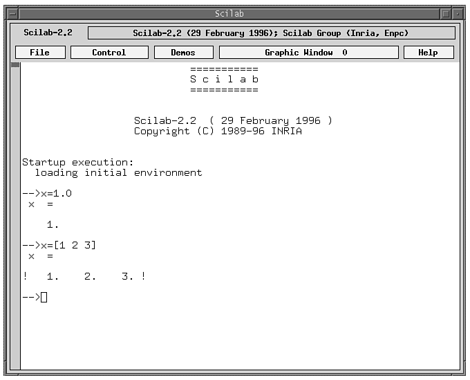
—>x=1.0

This sets x equal to 1.0. To declare an array, use square brackets:


—>x=[1 2 3]

x =

! 1. 2. 3. !

See Figure 35.1 to see what it looks like on your screen.

Figure 35.1. Main screen for Scilab.

To declare a large array you can use indices of the form [start:end]. Use a semicolon at the end of the line to indicate that you really do not want Scilab to echo the results back to you. So, the following statement


—>x=[1:100];

declares x as a vector of values from 1 to 100 and does not display the contents of x back to you. If you want to give staggered values of x, you can use an increment operator in the form [start:increment:stop]. So, this statement declares x to contain five odd numbers from 1:


—>x=[1:2:10]

x =

! 1. 3. 5. 7. 9. !

Let's try an example of a simple matrix multiplication problem of ax=b. First declare the a matrix, separating all the rows with semicolons. If you do not use semicolons, the values in matrix a will be interpreted as a 25´1 vector instead of a 5´5 matrix.


—>a=[ 1 1 0 0 0; 1 1 1 0 0; 0 1 1 1 0; 0 0 1 1 1; 0 0 0 1 1]

a =

! 1. 1. 0. 0. 0. !

! 1. 1. 1. 0. 0. !

! 0. 1. 1. 1. 0. !

! 0. 0. 1. 1. 1. !

! 0. 0. 0. 1. 1. !

Then declare X as a vector.


—>X=[ 1 3 5 7 9 ]

X =

! 1. 3. 5. 7. 9. !

To get the dimensions right for the multiplication, you have to use the single quotes ():Scilab multiplication;single quote operator () to get the transpose of X. Then put the results of the multiplication of a and X transpose into b.


—>b= a * X'

b =

! 4. !

! 9. !

! 15. !

! 21. !

! 16. !

—>

The results look right. In fact, Scilab displayed the dimensions correctly too, since the results of the multiplication are a matrix of size 5´1.

More Information on Scilab

The documentation for the Scilab application is available from ftp.inria.fr in the /INRIA/Projects/Meta2/Scilab/doc directory. It contains a PostScript document called intro.ps which contains the user's manual titled Introduction to Scilab. Take time to read this manual carefully.

Pari

The Pari package is useful for doing symbolic mathematical operations. Its primary features include an arbitrary precision calculator, its own programming facilities, and interfaces to C libraries.

Where To Get Pari

To get Pari, use the FTP site megrez.math.u-bordeaux.fr, and from the /pub/pari/unix directory get the gplinux.tar.gz file. The binaries may not work with a later version of Linux because the binaries are built with older versions of shared libraries. If you have a newer version of Linux than the one supported by Pari, either you can edit the sources yourself or wait until the authors of Pari catch up. Sorry.

With the version of Linux on the CD-ROM, you need to compile your own version of Pari. The source files are in the pari-1.39.03.tar.gz file. The source tar file unpacks into three directories: src, doc, and examples. You will find the examples very useful indeed.

To compile the sources, run the Makemakefile command in the src directory. When creating this version, remove the definition of the option -DULONG_NOT_DEFINED from the CFLAGS macro in the newly created Makefile. Then type make at the prompt. Be prepared to wait awhile for this package to compile.

Running Pari

After you have compiled the source files for Pari, type gp at the console prompt. Your prompt will be a question mark (?). Start by typing simple arithmetic expressions at this prompt. You should be rewarded with answers immediately. Let's look at the following sample session:


? 4*8

%1 = 32

? 4/7*5/6

%2 = 10/21

The answer was returned to us in fractions. To get real numbers, introduce just one real number in the equation. You will then get the answer as a real number. The percent signs identify the returned line numbers.


? 4.0/7 * 5/6

%3 = 0.4761904761904761904761904761

To set the precision in number of digits, you use the ?\precision command. The maximum number of digits is 315,623, a large number for just about all users. For a modest precision of 10 digits to the right of the decimal point, use


?\precision = 10

precision = 10 significant digits

? 4.0/7*5/6

%4 = 0.47619004761

You can even work with expressions, as shown in the following example:


? (x+2)*(x+3)

%5 = x^2+5*x + 6

You can assign values to variables to get the correct answer from evaluating an expression.


? x = 3

%6 = 3

? eval(%5)

%7 = 60

This is not where the power of Pari ends, though. You can factor numbers, solve differential equations, and even factor polynomials. The FTP site for Pari contains a wealth of information and samples. See megrez.math.u-bordeaux.fr. Also, the examples and docs directories contain samples and the manual to help you get started.

Using LISP-STAT

For statistical computing, consider using LISP-STAT. Written by Luke Tierney at the University of Minnesota, LISP-STAT is a very powerful, interactive, object-oriented LISP package.

Where To Get LISP-STAT

The LISP-STAT package is available from ftp.stat.umn.edu in the /pub/xlispstat directory. Get the latest tar file version you can—currently, xlispstat-3-44.tar.gz. In order to build this file you need the dld library for Linux. This dld library is found in tsx-11.mit.edu in the /pub/linux/binaries/libs directory as dld-3.2.5.bin.tar.gz. Install this dld library in the /lib directory first.

Running xlispstat

At the command prompt in an Xterm, type xlispstat. You will be presented with a > prompt. Type commands at this prompt. For example, to multiply two matrices together, use the command:


> (def a (matrix '(3 3) '(2 5 7 1 2 3 1 1 2)))

A

> (def b (matrix '(3 1) '(4 5 6)))

B

> (matmult a b)

#2A((75.0) (32.0) (21))

The variables in LISP-STAT are not case-sensitive. Note the single quote (') before the list of numbers for the matrix. If you omit the quote, the list will be evaluated and replaced with the result of the evaluation. By leaving the single quote in there, you are forcing the interpreter to leave the list in its place.

Let's try solving a simple set of linear equations using LISP-STAT. The following would be a simple example to solve:


3.8x + 7.2y = 16.5

1.3x - 0.9y = -22.1

The following script would set up and solve this linear equation problem:


> (def a (matrix '(2 2) '(3.8 7.2 1.3 -0.9)))

A

> (def b (matrix '(2 1) '(16.5 -22.1)))

B

> (matmult (inverse a) b)

#2A((-11.288732394366198) (8.249608763693271))

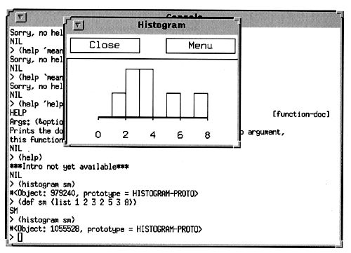
You can do other math operations on lists of numbers as well. See the following example for calculating the mean of a list of numbers:


> (def sm (list 1.1 2.3 4.1 5.7 2.1))

SM

> (mean SM)

3.06

There are many plotting functions available for LISP-STAT. For plotting one variable, try the function plot-function. For (x,y) pairs of numbers, use the plot-lines function. For a function of two variables, use the spin-function. For 3-D plots, use the spin-plot function.

Plots are not limited to lines. You can do histograms, planar plots, and so on. See the help pages for details on specifics of how to generate these plots. Two or more plots can be linked together so that changes in one set of data can be reflected in another. You can add points to a plot using the add-points function. For reconfiguring how the points are displayed, you can send commands to the plot windows. Plots can be linked together to enable more than one view of the same data.

Figure 35.2 A Histogram sample

Each plot is displayed in an X window. You can move the mouse cursor over a point, and it will echo back a value for you.

To get help on this system, use the help command. The help documentation for this command should be visible. If nothing shows up, check the environment variables to see if the binaries are in the PATH.

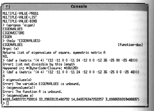
Figure 35.3 Sample of using EIGEN-VALUES

A Last Note

For simple math operations involving spreadsheets, you can always use the xspread program provided with the X package. (The CD-ROM at the back of the guide has version 2.1.) For more powerful spreadsheet functions, you might want to resort to a commercial spreadsheet package and take advantage of its support, too. The XESS spreadsheet is available for Linux from Applied Information systems, (919) 942-7801 or http://www.ais.com/Xess. You can share data between spreadsheets, or use the API to develop and have access to a full suite of math functions available on spreadsheets that run under DOS or UNIX.

Wolfram Research has released its Mathematica program for Linux. The Mathematica package has extensive numeric and symbolic capabilities, 2-D and 3-D graphics, and a very large library of application programs. With an additional feature called MathLink, you can exchange information between other applications on a network. You can get more information about Mathematica from info@wri.com or http://www.wri.com.

Summary

You have several options when it comes to performing mathematical operations or writing such applications under Linux. You can either write the code yourself using C, FORTRAN, or other available languages—or you can use a package. If you are familiar with MATLAB, consider using Scilab. For regular expressions and polynomials, try using Pari. If you are a LISP user or want to do vector operations or statistics, consider using the LISP-STAT package.